
Until this point in class, we have used a very simple model of memory: given an address, we either read a value from or wrote a value to the memory cell at that address. In this unit, we're going to consider real memory systems, which are comprised of a hierarchy of storage devices with different capacities, costs, and time to access.
Think of books as the data you'd like to store and access during your life. I have a few (say 3-6) books on my office desk. If I stand up and take a few steps, I get access more books (~60), which I keep on the shelves in my office. But sometimes, I want books that I don't have in my office, and that's when I leave my office and walk to Widener Library, which contains lots more books (~3.5 million) on its shelves. The Harvard Depository holds even more books (~10 million), which I can have delivered to my office if I'm willing to wait a day or so. Finally, if I can't find what I want in the Harvard Library system, I can access BorrowDirect, a consortium of 13 Ivy+ institutions that make the books in their library systems available to the students and faculty of its members. Through BorrowDirect, I have access to yet more books (~90 million), but it will take about 4 days to a book to arrive from BorrowDirect.
This hierarchy of libraries is similar in nature to the hierarchy of storage in our computing systems. Different levels have different capacities, costs, and times to access.
What maps to each of these layers in a computer's storage system?
| For books | For data | Comments |
|---|---|---|
| my desk | processor's registers | where most work is done |
| my shelves | processor's caches | where frequently accessed data is kept |
| Widener | main memory | main, active storage for the computer/university |
| Harvard Depository | hard disk or flash storage | archival storage |
| BorrowDirect | networked storage | data out in the world |
Why don't we connect the processor directly to main memory (or flash
memory or a hard disk)? We certainly code encode an instruction, as
we saw in the Assembly Unit, to read and write directly to main memory
(e.g., addq A, B). That's not a problem. The problem comes when we
start thinking about how long it will take to access the value stored
at address A and how much it will cost us to build a fast storage
system with a large capacity.
Let's look at what it would cost me to buy extra storage for my MacBook Pro from apple.com (October 2019).
| Storage Technology | Size (GB) | Cost ($) | $/GB | Access Time |
|---|---|---|---|---|
| DDR4 DRAM (memory) | 16 | $400 | $25 | ~12-15 ns |
| SSD flash | 256 | $200 | $0.80 | 0.1 ms |
| Hard drive | 2048 | $100 | $0.05 | 12 ms |
Notice that it would cost about $50,000 to build a 2 Terabyte main memory out of DDR4 DRAM chips, or I could just buy a $100 hard drive.
Here's the key point: We cannot build a storage system from a single type of digital technology that is simultaneously big, fast, and cheap. So instead, our goal is to create a storage system made up of layers of different storage technologies that gives the appearance of being big and fast. It will cost a bit more than a big and slow storage system, but it will also cost a lot less than a big and fast one.
How do we accomplish this? Well, let's return to our books analogy. What do I keep nearby? Two types of books: (a) books that I am personally writing; and (b) books that I frequently reference (i.e., read). With this in mind, what should a processor keep nearby? Data that it writes (creates) and data that it frequently references (reads)!
The Principle of Locality of Reference
This brings us to the concept of locality of reference. Programs that run fast on modern computing systems exhibit two types of locality of reference. Let's consider the following procedure when thinking about concrete examples of the two types of locality of reference:
```c++ long f (const int* v, int n) {
long sum = 0;
for (int i = 0; i < n; ++1) {
    sum += v[i];
}
return sum;
} ````
The first is temporal locality. A program exhibits temporal
locality if when referencing a memory location, the program will
likely access that location again in the not-too-distant future. The
variables i, sum, and v[] all exhibit good temporal locality in
the loop, as do the loop instructions.
Note that the elements in the array v don't individually exhibit
temporal locality. Each is accessed on only one of the n loop
iterations. However, because of the sequential nature of the accesses
to the elements in v, this array exhibits good spatial locality
during the execution of this loop. A program exhibits spatial
locality if when referencing a memory location, the program will
likely access a nearby location in the not-too-distant future.
Straightline code (without jumps or calls) exhibits good spatial
locality.
Caches
If a program exhibits good locality of reference, we can use a technique called caching to make a memory system comprised of a hierarchy of storage devices to appear to be large and fast. In particular, when we build a cache, we use a small amount of relatively fast storage at one level of the memory hierarchy to speed up access to a large and relatively slow storage at the next higher level of the memory hierarchy. By "higher" we mean farther from the processor.
Simply stated, a cache works by storing copies of data whose primary home is on slower storage. A processor accesses data faster when a it’s located “nearby,” in fast storage.
Caches abound in computer systems; sometimes it seems like caching is the only performance-improving idea in systems. Processors have caches for primary memory. The operating system uses most of primary memory as a cache for disks and other stable storage devices. Running programs reserve some of their private memory to cache the operating system’s cache of the disk.
People have made a career of proposing different variants of caches for different use cases. When a program processes a file, the actual computation is done using registers, which are caching values from the processor cache, which is caching data from the running program’s memory, which is caching data from the operating system, which is caching data from the disk. And modern disks contain caches inside their hardware too!
Caches also abound in everyday life. Imagine how life would differ without, say, food storage—if every time you felt hungry you had to walk to a farm and eat a carrot you pulled out of the dirt. Your whole day would be occupied with finding and eating food! Instead, your refrigerator (or your dorm’s refrigerator) acts as a cache for your neighborhood grocery store, and that grocery store acts as a cache for all the food producers worldwide. Caching food is an important aspect of complex animals’ biology too. Your stomach and intestines and fat cells act as caches for the energy stored in the food you eat, allowing you to spend time doing things other than eating. And your colon and bladder act as caches for the waste products you produce, allowing you to travel far from any toilet.
(Link not about caches: Anna’s Since Magic Show Hooray!)
File I/O
In this unit, we are going to focus on caches that sit among the layers of the memory hierarchy from the main memory out through stable storage devices like disks and flash storage.
The problem set focuses on file I/O—that is, input and output (“I” and
“O”) for files. You’re likely familiar with files already. The stdin,
stdout, and stderr objects in C are references to files, as are C++’s
std::cin, std::cout, and std::cerr. C library functions like fopen,
fread, fprintf, fscanf, and fclose all perform operations on files.
These library routines are part of a package called standard I/O or
stdio for short. They are implemented in terms of lower-level
abstractions; the Linux/Mac OS X versions are called file descriptors,
which are accessed using system calls such as open, read, and write.
Although file descriptors and system calls are often hidden from programmers
by stdio, we can also access them directly.
Formally, a Unix file is simply a sequence of bytes. All I/O devices (e.g., disks, keyboards, displays, and networks) are modeled as files. This simple abstraction turns out to be extremely elegant and powerful. It, for instance, hides much of the difficult details of individual technologies from user programs.
We used simple I/O benchmark programs to evaluate the real-world impact of caches. Specifically, we ran several programs that write data to disk—my laptop’s SSD drive, via my virtual machine. These programs accomplish the same goal, but in several different ways.
w01-syncbytewrites the file (1) one byte at a time, (2) using direct system calls (write), (3) synchronously to the disk.“Synchronously” means that each
writeoperation completes only when the data has made its way through all layers of caching out to the true disk hardware. (At least that’s what it should mean!) We request synchronous writes by opening the file with theO_SYNCoption toopen.On my laptop,
w01-syncbytecan write about 2,400 bytes per second (it varies).w03-bytewrites the file (1) one byte at a time, (2) using direct system calls (write), (3) asynchronously—in other words, allowing the operating system to use its caches.On my laptop,
w03-bytecan write about 870,000 bytes per second—360x more thanw01-syncbyte!w05-stdiobytewrites the file (1) one byte at a time, (2) using stdio library function calls (fwrite), (3) asynchronously.On my laptop,
w05-stdiobytecan write about 52,000,000 bytes per second—22,000x more thanw01-syncbyte!
Even though all three programs write one byte at a time, caching makes the
fastest one 22,000x faster. The w05-stdiobyte program uses two distinct
layers of software cache: a stdio cache, managed by the stdio library
inside the program, uses caching to reduce the cost of system calls; and the
buffer cache, managed by the operating system inside the kernel, uses
caching to reduce the cost of disk access. The combination of these is
22,000x.
Buffer cache
With today’s machines and operating systems, the buffer cache ends up occupying much of the machine’s memory. It can hold data for many files, and for many drives and sources of storage, simultaneously.
Here’s what happens at a high level when w03-byte writes bytes to the file:
The application makes a
writesystem call asking the operating system to write a byte.The operating system performs this write to the buffer cache.
The operating system immediately returns to the application!
That is, the application gets control back before the data is written to disk. The data is written to disk eventually, either after some time goes by or because the buffer cache runs out of room, but such later writes can be overlapped with other processing.
Stdio cache
But w03-byte is still much slower than it needs to be, because it
performs many expensive operations—namely [system calls]system
calls. These operating system invocations are slow, as we saw in the
last Unit, because they require the processor to save its state,
switch contexts to the kernel, process arguments, and then switch
back. Another layer of caching, the stdio cache, can get rid of
these system calls. The stdio cache is a cache in application
memory for the buffer cache, which is in kernel memory.
Here’s what happens at a high level when w05-stdiobyte writes bytes
to the file:
The application makes an
fwritelibrary function call asking the stdio library to write a byte.The library performs this write to its cache and immediately returns to the application.
That is, the application gets control back even before a system call is made. The data is written out of the stdio cache using a system call eventually, either when the stdio cache runs out of room, it is explicitly flushed, or the program exits.
Big blocks and cached reads
If we think about what's happening in the abstract, the stdio and buffer caches are allowing the process to skip waiting for its writes to disk to complete. The caches guarantee that the writes will complete eventually, and the process doesn't need to worry about when. (We'll revisit this simple assumption later when we start thinking about consistency and coherence.)
Does caching work for reads as well as writes? Yes! Unlike a disk write, the process cannot continue its execution without the data returned from a disk read. If a program's execution exhibits temporal locality, caching the first read of an address means that we do not have to wait on later reads of that same address. Furthermore, if the program's execution also exhibits spatial locality, the cache can grab a big block of data on the first read -- bigger than the size of the read request -- and eliminate subsequent reads to disk that are around the address of the first read request.
We can use this approach of using big blocks in transferring data
between the cache and the slower storage (e.g., a disk) to improve the
performance of writes too. The programs w0[2,4,6]-*.cc write
512-byte blocks to disk, rather than single bytes. In particular,
w02-syncblockwrites the file (1) 512 bytes at a time, (2) using system calls, (3) synchronously to the disk. On my laptop, it can write about 1,300,000 bytes per second. This program is about 512x faster thanw01-syncbyte, as would be expected given that it writes 511 more bytes per slow write thanw01-syncbyte.w04-blockwrites the file (1) 512 bytes at a time, (2) using system calls, (3) asynchronously. On my laptop, it can write about 200,000,000 bytes per second.w06-stdioblockwrites the file (1) 512 bytes at a time, (2) using stdio, (3) asynchronously. On my laptop, it can write about 270,000,000 bytes per second—112,500x more thanw01-syncbyte!
We then used strace to look more deeply at the operation of these
programs and their interaction with the stdio and buffer caches. You
can read more about strace in the
section notes.
Latency and throughput
So far, we have been categorizing the performance of a storage device by talking about its latency, i.e., the time it takes to satisfy a read or write request. While this is an important measure, it is not the only important performance measure for many I/O devices.
The second imporant performance measure for many I/O devices is throughput (also called bandwidth), which characterizes the number of read or write operations that an I/O device can complete per second. For latency measures, lower numbers are better. For throughput measures, higher numbers are better.
Consider a typical disk drive. Today, these I/O devices have an average latency of about 5 milliseconds. Turning that into a throughput number, you could write bytes to random locations in a large disk file at rate of about 1 MB per second. However, today's disk drives have a maximum transfer rate (i.e., throughput) of about 150 MB per second. The higher throughput occurs when you write many consecutive bytes to a disk file.
To understand the difference, you need to understand that latency is both a distance effect and a technology effect for some storage devices, like disk drives, magnetic tapes, and even flash memories in a way. Sticking with disk drives, latency grows as we move down the memory hierarchy simply because the physical distance grows between the processor and the I/O devices lower in the hierarchy. The farther a request has to travel electrically, the longer it takes.
Once the request reaches a disk drive, the mechanical aspects of the disk drive's configuration introduce additional latency. A disk drive is comprised of one or more platters (picture a CDROM in your mind) stacked on a spindle. This spindle rotates the platters at an example speed of 7200 revolutions per minute (RPM). To read or write bits on a disk drive's platter, an electronic head is placed on the end of an arm, which moves back and forth over the platter, just barely above its surface. To write a bit, the arm needs to mechanically move somewhere along a radius from the spindle to the edge of the platter, and then the platter has to spin to the right location. Then a bit is read or written. I get tired just explaining all these steps.
However, notice what happens once disk drive head gets to the right location. The head can read and write a whole bunch of bits by simply letting the platter spin below it. This is why reading (or writing) a whole bunch of bits sequentially is so much faster than randomly writing bits all over the disk's platters.
Latency Numbers Every Programmer Should Know
Aside: Synchronous writes in depth on a flash drive
If you want to know what happens in a flash drive, read this section. If not, feel free to skip to the next section.
Let's assume that we are running w01-syncbyte. Here’s what happens
at a high level when that application writes bytes to the file located
on my computer's flash drive:
The application makes a
writesystem call asking the operating system to write a byte.The operating system performs this write to its cache. But it also observes that the written file descriptor requires synchronous writes, so it begins the process of writing to the drive--in my case, an SSD.
This drive cannot write a single byte at a time! Most storage technologies other than primary memory read and write data in contiguous blocks, typically 4,096 or 8,192 bytes big. So for every 1-byte application write, the operating system must write an additional 4,095 surrounding bytes, just because the disk forces it to!
That 4,096-byte write is also slow, because it induces physical changes. The job of a disk drive is to preserve data in a stable fashion, meaning that the data will outlast accidents like power loss. On today’s technology, the physical changes that make data stable take more time than simple memory writes.
But that’s not the worst part. SSD drives have a strange feature where data can be written in 4KiB or 8KiB units, but erasing already-written data requires much larger units—typically 64KiB or even 256KiB big! The large erase, plus other SSD features like “wear leveling,” may cause the OS and drive to move all kinds of data around: our 1-byte application write can cause 256KiB or more traffic to the disk. This explosion is called write amplification.
So the system call only returns after 4–256KiB of data is written to the disk.
Stable and volatile storage
Computer storage technologies can be either stable or volatile.
Stable storage is robust to power outages. If the power is cut to a stable storage device, the stored data doesn’t change.
Volatile storage is not robust to power outages. If the power is cut to a volatile storage device, the stored data is corrupted and usually considered totally lost.
Registers, SRAM (static random-access memory—the kind of memory used for processor caches), and DRAM (dynamic random-access memory—the kind of memory used for primary memory) are volatile. Disk drives, including hard disks, SSDs, and other related media are (relatively) stable.
Aside: Stable DRAM?
Interestingly, even DRAM is more stable than once thought. If someone wants to steal information off your laptop’s memory, they might grab the laptop, cool the memory chips to a low temperature, break open the laptop and transplant the chips to another machine, and read the data there.
Here’s a video showing DRAM degrading after a power cut, using the Mona Lisa as a source image.
High throughput, high latency
The best storage media have low latency and high throughput: it takes very little time to complete a request, and many units of data can be transferred per second.
Latency and throughput are not, however, simple inverses: a system can have high latency and high throughput. A classic example of this is “101Net,” a high-bandwidth, high-latency network that has many advantages over the internet. Rather than send terabytes of data over the network, which is expensive and can take forever, just put some disk drives in a car and drive it down the freeway to the destination data center. The high information density of disk drives makes this high-latency, high-throughput channel hard to beat in terms of throughput and expense for very large data transfers.
101Net is a San Francisco version of the generic term sneakernet. XKCD took it on.
Amazon Web Services offers physical-disk transport; you can mail them a disk using the Snowball service, or if you have around 100 petabytes of storage (that’s roughly 1017 bytes!!?!?!?!?!) you can send them a shipping container of disks on a truck. Look, here it is.

“Successful startups, given the way they collect data, have exabytes of data,” says the man introducing the truck, so the truck is filled with 1017 bytes of tracking data about how long it took you to favorite your friend’s Pokemon fashions or whatever.
Historical costs of storage
We think a lot in computer science about costs: time cost, space cost, memory efficiency. And these costs fundamentally shape the kinds of solutions we build. But financial costs also shape the systems we build--in some ways more fundamentally--and the costs of storage technologies have changed at least as dramatically as their capacities and speeds.
This table gives the price per megabyte of different storage technologies, in price per megabyte (2010 dollars), up to 2018.
| Year | Memory (DRAM) | Flash/SSD | Hard disk |
|---|---|---|---|
| ~1955 | $411,000,000 | $6,230 | |
| 1970 | $734,000.00 | $260.00 | |
| 1990 | $148.20 | $5.45 | |
| 2003 | $0.09 | $0.305 | $0.00132 |
| 2010 | $0.019 | $0.00244 | $0.000073 |
| 2018 | $0.0059 | $0.00015 | $0.000020 |
The same costs relative to the cost of a hard disk in ~2018:
| Year | Memory | Flash/SSD | Hard disk |
|---|---|---|---|
| ~1955 | 20,500,000,000,000 | 312,000,000 | |
| 1970 | 36,700,000,000 | 13,000,000 | |
| 1990 | 7,400,000 | 270,000 | |
| 2003 | 4,100 | 15,200 | 6.6 |
| 2010 | 950 | 122 | 3.6 |
| 2018 | 29.5 | 7.5 | 1 |
These are initial purchase costs and don’t include maintenance or power. DRAM uses more energy than hard disks, which use more than flash/SSD. (Prices from here and here. $1.00 in 1955 had “the same purchasing power” as $9.45 in 2018 dollars.)
There are many things to notice in this table, including the relative changes in prices over time. When flash memory was initially introduced, it was 2300x more expensive per megabyte than hard disks. That has dropped substantially; and that drop explains why large amounts of fast SSD memory is so ubiquitous on laptops and phones.
Hard disks
The performance characteristics of hard disks are particularly interesting. Hard disks can access data in sequential access patterns much faster than in random access patterns. (More on access patterns) This is due to the costs associated with moving the mechanical “head” of the disk to the correct position on the spinning platter. There are two such costs: the seek time is the time it takes to move the head to the distance from the center of the disk, and the rotational latency is the time it takes for the desired data to spin to underneath the head. Hard disks have much higher sequential throughput because once the head is in the right position, neither of these costs apply: sequential regions of the disk can be read as the disk spins. This is just like how a record player plays continuous sound as the record spins underneath the needle. A typical recent disk might rotate at 7200 RPM and have ~9ms average seek time, ~4ms average rotational latency, and 210MB/s maximum sustained transfer rate. (CS:APP3e)
The storage hierarchy (revisited)
Hopefully, you're starting to better understand what we mean by storage hierarchy and how different technologies fit into it.
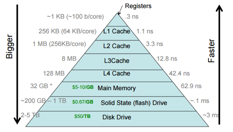
The storage hierarchy shows the processor caches divided into multiple levels, with the L1 cache (sometimes pronounced “level-one cache”) closer to the processor than the L4 cache. This reflects how processor caches are actually laid out, but we often think of a processor cache as a single unit.
Different computers have different sizes and access costs for these hierarchy levels; the ones above are typical, but here are some more, based on those for my desktop iMac, which has four cores (i.e., four independent processors): ~1KB of registers; ~9MB of processor cache; 8GB primary memory; 512GB SSD; and 2TB hard disk. The processor cache divides into three levels. There are 128KB of L1 cache, divided into four 32KB components; each L1 cache is accessed only by a single core, which makes accessing it faster, since there’s no need to arbitrate between cores. There are 512KB of L2 cache, divided into two 256KB components (one per “socket”, or pair of cores). And there are 8MB of L3 cache shared by all cores.
And distributed systems have yet lower levels. For instance, Google and Facebook have petabytes or exabytes of data, distributed among many computers. You can think of this as another storage layer, networked storage, that is typically slower to access than HDDs.
Each layer in the storage hierarchy acts as a cache for the following layer.
Cache model
We describe a generic cache as fast storage that is divided into slots:
- Each slot is capable of holding data from slow storage (from farther down the storage hierarchy).
- A slot is empty if it contains no data. It is full if it contains data from slow storage.
- Each slot has a name (for instance, we might refer to “the first slot” in a cache).
Slow storage is divided into blocks such that:
- Each block can fit in a slot.
- Each block has an address.
- If a cache slot (in fast storage) is full, meaning it holds data from a block (in slow storage), it must also know the address of that block.
There are some terms that are used in the contexts of specific levels in the hierarchy; for instance, a cache line is a slot in the processor cache (or, sometimes, a block in memory).
Read caches must respond to user requests for data at particular addresses. On each access, a cache typically checks whether the specified block is already loaded into a slot. If it is, the cache returns that data; otherwise, the cache first loads the block into some slot, then returns the data from the slot.
A cache access is called a hit if the data is already loaded into a cache slot, and a miss otherwise. Cache hits are good because they are cheap. Cache misses are bad: they incur both the cost of accessing the cache and the cost of accessing the slower storage. We want most accesses to hit. That is, we want a high hit rate, where the hit rate is the fraction of accesses that hit.
Eviction policies and reference strings
When a cache becomes full, we may need to evict data currently in the cache to accommodate newly required data. The policy the cache uses to decide which existing slot to vacate (or evict) is called the eviction policy.
We can reason about different eviction policies using sequences of addresses called reference strings. A reference string represents the sequence of blocks being accessed by the cache’s user. For instance, the reference string “1 2 3 4 5 6 7 8 9” represents nine sequential accesses.
For small numbers of slots, we can draw how a cache responds to a reference string for a given number of slots and eviction policy. Let’s take the reference string “1 2 3 4 1 2 5 1 2 3 4 5”, and an oracle eviction policy that makes the best possible eviction choice at every step. Here’s how that might look. The cache slots are labeled with Greek letters; the location of an access shows what slot was used to fill that access; and misses are circled.
| 1 | 2 | 3 | 4 | 1 | 2 | 5 | 1 | 2 | 3 | 4 | 5 | |
|---|---|---|---|---|---|---|---|---|---|---|---|---|
| α | ① | 1 | 1 | ③ | ||||||||
| β | ② | 2 | 2 | ④ | ||||||||
| γ | ③ | ④ | ⑤ | 5 |
Some notes on this diagram style: At a given point in time (a given column), read the cache contents by looking at the rightmost numbers in or before that column. The least-recently-used slot has the longest distance to the most recent reference before the column. And the least-recently-loaded slot has the longest distance to the most recent miss before the column (the most recent circled number).
The hit rate is 5/12.
What the oracle’s doing is the optimal cache eviction policy: Bélády’s optimal algorithm, named after its discoverer, László Bélády (the article). This algorithm selects for eviction a slot whose block is used farthest in the future (there might be multiple such slots). It is possible to prove that Bélády’s algorithm is optimal: no algorithm can do better.
Unfortunately, it is possible to use the optimal algorithm only when the complete sequence of future accesses is known. This is rarely possible, so operating systems use other algorithms instead.
LRU
The most common algorithms are variants of Least Recently Used (LRU) eviction, which selects for eviction a slot that was least recently used in the reference string. Here’s LRU working on our reference string and a three-slot cache.
| 1 | 2 | 3 | 4 | 1 | 2 | 5 | 1 | 2 | 3 | 4 | 5 | |
|---|---|---|---|---|---|---|---|---|---|---|---|---|
| α | ① | ④ | ⑤ | ③ | ||||||||
| β | ② | ① | 1 | ④ | ||||||||
| γ | ③ | ② | 2 | ⑤ |
LRU assumes locality of reference (temporal locality): if we see a reference to a location, then it’s likely we will see another reference to the same location soon.
FIFO
Another simple-to-specify algorithm is First-In First-Out (FIFO) eviction, also called round-robin, which selects for eviction the slot that was least recently evicted. Here’s FIFO on our reference string.
| 1 | 2 | 3 | 4 | 1 | 2 | 5 | 1 | 2 | 3 | 4 | 5 | |
|---|---|---|---|---|---|---|---|---|---|---|---|---|
| α | ① | ④ | ⑤ | 5 | ||||||||
| β | ② | ① | 1 | ③ | ||||||||
| γ | ③ | ② | 2 | ④ |
Larger caches
We normally expect that bigger caches (i.e., ones with more slots) work better (i.e., achieve higher hit rates). If a cache has more slots, it can hold a greater proportion of the blocks in a process's reference string, which often translates into a higher hit rate. While this is generally true, it not always! Here we raise the number of slots to 4 and evaluate all three algorithms.
| 1 | 2 | 3 | 4 | 1 | 2 | 5 | 1 | 2 | 3 | 4 | 5 | |
|---|---|---|---|---|---|---|---|---|---|---|---|---|
| α | ① | 1 | 1 | ④ | ||||||||
| β | ② | 2 | 2 | |||||||||
| γ | ③ | 3 | ||||||||||
| δ | ④ | ⑤ | 5 |
| 1 | 2 | 3 | 4 | 1 | 2 | 5 | 1 | 2 | 3 | 4 | 5 | |
|---|---|---|---|---|---|---|---|---|---|---|---|---|
| α | ① | 1 | 1 | ⑤ | ||||||||
| β | ② | 2 | 2 | |||||||||
| γ | ③ | ⑤ | ④ | |||||||||
| δ | ④ | ③ |
| 1 | 2 | 3 | 4 | 1 | 2 | 5 | 1 | 2 | 3 | 4 | 5 | |
|---|---|---|---|---|---|---|---|---|---|---|---|---|
| α | ① | 1 | ⑤ | ④ | ||||||||
| β | ② | 2 | ① | ⑤ | ||||||||
| γ | ③ | ② | ||||||||||
| δ | ④ | ③ |
The optimal and LRU algorithms’ hit rates improved, but FIFO’s hit rate dropped!
This is called Bélády’s anomaly (the same Bélády): for some eviction algorithms, hit rate can decrease with increasing numbers of slots. FIFO suffers from the anomaly. But even some simple algorithms do not: LRU is anomaly-proof.
The argument is pretty simple: Adding a slot to an LRU cache will never turn a hit into a miss, because if an N-slot LRU cache and an (N+1)-slot LRU cache process the same reference string, the contents of the N-slot cache are a subset of the contents of the (N+1)-slot cache at every step. This is because for all N, an LRU cache with N slots always contains the N most-recently-used blocks—and the N most-recently-used blocks are always a subset of the N+1 most-recently-used blocks.
Implementing eviction policies
The cheapest policy to implement is FIFO, because it doesn’t keep track of any facts about the reference string (the least-recently-evicted slot is independent of reference string). LRU requires the cache to remember when slots were accessed. This can be implemented precisely, by tracking every access, or imprecisely, with sampling procedures of various kinds. Bélády’s algorithm can only be implemented if the eviction policy knows future accesses, which requires additional machinery—either explicit information from cache users or some sort of profiling information.
You can play with different eviction policies and cache configurations using
the cache.cc code distributed in cs61-lectures/storage3.
Cache associativity
Let's a consider a cache with S total slots, each capable of holding a block of slow storage.
In a fully-associative cache, any block can be held in any slot.
In a set-associative cache, the block with address A can fit in a subset of the slots called C(A). For example, in a two-set associative cache, a block with address A can be held in one of two slots and |C(A)| = 2.
In a direct-mapped cache, each block can fit in exactly one slot. For example, a cache might require that the block with address A go into slot number (A mod S).
Fully-associative and direct-mapped caches are actually special cases of set-associative caches. In a fully-associative cache, C(A) always equals the whole set of slots. In a direct-mapped cache, C(A) is always a singleton.
Another special case is a single-slot cache. In a single-slot cache, S = 1: there is only one slot. A single-slot cache fits the definition of both direct-mapped and fully-associative caches: each block with address A can go into exactly one slot, and any block can be held in that single slot. The stdio cache is a single-slot cache.
Single-slot caches and unit size
You might think that single-slot caches are useless unless the input reference string has lots of repeated blocks. But this isn’t so because caches can also change the size of data requested. This effectively turns access patterns with few repeated accesses into access patterns with many repeated accesses, e.g., if the cache’s user requests one byte at a time but the cache’s single slot can contain 4,096 bytes. (More in section notes)
Consider reading, for example. If the user only requests 1 byte at a time, and the cache reads 4096 bytes, then the 4095 subsequent reads by the application can be easily fulfilled from the cache, without reaching out again to the file system.
On the other hand, if the user reads more than 4,096 bytes at once, then a naively-implemented stdio cache might have unfortunate performance. It might chunk this large read into some number of 4,096 byte reads. This would result in the stdio library making more system calls than absolutely necessary.
Random-access files, streams, and file positions
One of the Unix operating system’s big ideas was the unification of two different kinds of I/O into a single “file descriptor” abstraction. These kinds of I/O are called random-access files and streams. Metaphorically, random-access files are like books and streams are like the stories my grandmother used to tell me.
A random-access file has a finite length, called its size. It is possible to efficiently skip around inside the file to read or write at any position, so random-access files are seekable. It is also often possible to map the file into memory (see below). A random-access file is like an array of bytes.
A stream is a possibly-infinite sequence of bytes. It is not possible to
skip around inside a stream. A stream is more like a queue of bytes: a
stream writer can only add more bytes to the end of the stream, and a stream
reader can only read and remove bytes from the beginning of the stream.
Streams are not seekable or mappable. The output of a program is generally a
stream. (We used yes as an example.)
Some previous operating systems offered fundamentally different abstractions. Unix (like some other OSes) observed that many operations on random-access files and streams can have essentially similar semantics if random-access files are given an explicit feature called the file position. This is a file offset, maintained by the kernel, that defines the next byte to be read or written.
When a random-access file is opened, its file position is set to 0, the
beginning of a file. A read system call that reads N bytes advances the
file position by N, and similarly for write. An explicit seek system
call is used to change the file position. When the file position reaches the
end of the file, read will return 0.
Streams don’t have file positions—the seek system call will return -1 on
streams. Instead, a read system call consumes the next N bytes from the
stream, and a write system call adds N bytes to the end of the stream.
When the read system call reaches the end of the stream (which only happens
after the write end is closed), it will return 0.
What’s important here is that a sequence of read system calls will return
the same results given a random-access file or a stream with the same
contents. And similarly, a sequence of write system calls will produce the
same results whether they are directed to a random-access file or a stream.
Programs that simply read their inputs sequentially and write their outputs
sequentially—which are most programs!—work identically on files and streams.
This makes it easy to build very flexible programs that work in all kinds of
situations.
(But special system calls that work on specific file offsets are useful for
random-access files, and now they exist: see pread(2) and pwrite(2).)
Read caches
The r* programs in cs61-lectures/storage3 demonstrate different mechanisms
for reading files.
r01-directsectorreads the file (1) 512 bytes at a time (this unit is called a sector), (2) using system calls (read), (3) synchronously from the disk. TheO_DIRECTflag disables the buffer cache, forcing synchronous reads; whenO_DIRECTis on, the application can only read in units of 512 bytes.On my laptop,
r01-directsectorcan read about 7,000,000 bytes per second.r02-sectorreads the file (1) 512 bytes at a time, (2) using system calls, (3) asynchronously (allowing the operating system to use the buffer cache).On my laptop,
r02-sectorcan read somewhere around 360,000,000 bytes per second (with a lot of variability).r07-stdioblockreads the file (1) 512 bytes at a time, (2) using stdio, (3) asynchronously.On my laptop,
r07-stdioblockcan read somewhere around 480,000,000 bytes per second (with a lot of variability).r03-bytereads the file (1) one byte at a time, (2) using system calls, (3) asynchronously.On my laptop,
r03-bytecan read around 2,400,000 bytes per second.r05-stdiobytereads the file (1) one byte at a time, (2) using stdio, (3) asynchronously.On my laptop,
r05-stdiobytecan read around 260,000,000 bytes per second.
These numbers give us a lot of information about relative costs of different
operations. Reading direct from disk is clearly much faster than writing
direct to disk. (Of course this might also be impacted by the virtual machine
on which we run.) And this also gives us some feeling for the cost of system
calls: reading a byte at a time is about 150x slower than reading 512 bytes at
a time. Assuming we knew the cost of the rest of the r* programs (i.e., the
costs of running the loop and occasionally printing statistics, which are
about the same for all programs), then this information would let us deduce
the R and U components of system call costs.
Reverse reading
Some r* programs feature different access patterns.
r08-revbytereads the file (0) in reverse, (1) one byte at a time, (2) using system calls, (3) asynchronously. On my laptop, it reads about 1,400,000 bytes per second.r09-stdiorevbytereads the file (0) in reverse, (1) one byte at a time, (2) using stdio, (3) asynchronously. On my laptop, it reads about 3,500,000 bytes per second—more than twice as much!
We used strace to examine the system calls made by
r09-stdiorevbyte. We discovered the stdio uses an aligned cache for
reads. This means that, for reads, the stdio cache always aligns its cache so
that the first offset in the cache is a multiple of the cache size, which is
4,096 bytes. This aligned cache is quite effective for forward reads and for
reverse reads; in both cases, stdio’s prefetching works.
Stdio doesn’t work great for all access patterns. For example, for random one-byte reads distributed through in a large file, stdio will each time read 4,096 bytes, only one of which is likely to be useful. This incurs more per-unit costs than simply accessing the bytes directly using one-byte system calls.
The stdio cache is aligned for reads, but is it for writes? Check out the
strace results for w10-stdiorevbyte to find out. You can do better than
stdio here, at the cost of some complexity.
Memory mapping
Why is the stdio cache only 4,096 bytes? One could make it bigger, but very large stdio caches can cause problems by crowding out other data. Imagine an operating system where many programs are reading the same large file. (This isn’t crazy: shared library files, such as the C++ library, are large and read simultaneously by most or all programs.) If these programs each have independent copies of the file cached, those redundant copies would mean there’s less space available for the buffer cache and for other useful data.
The neat idea of memory-mapped I/O allows applications to cache files without redundancy by directly accessing the operating system’s buffer cache.
The relevant system calls are mmap(2) and munmap(2). mmap tells the
operating system to place a region of a file into the application’s heap. But
unlike with read, this placement involves no copying. Instead, the operating
system plugs the relevant part of the buffer cache into that part of the
application’s heap! The application is now sharing part of the buffer cache.
The application can “read” or “write” the file simply by accessing that heap
region.
r16-mmapbytereads the file (1) one byte at a time, (2) usingmmap, (3) asynchronously (the operating system takes care of prefetching, batching, and, for writes, write coalescing). On my laptop, it reads about 350,000,000 bytes per second—more even than stdio!
Memory mapping is very powerful, but it has limitations. Streams cannot be
memory mapped: memory mapping only works for random-access files (and not even
for all random-access files). Memory mapping is a little more dangerous; if
your program has an error and modifies memory inappropriately, that might now
corrupt a disk file. (If your program has such an error, it suffers from
undefined behavior and could corrupt the file anyway, but memory mapping does
make corruption slightly more likely.) Finally, memory mapping has far nastier
error behavior. If the operating system encounters a disk error, such as “disk
full”, then a write system call will return −1, which gives the
program a chance to clean up. For a memory-mapped file, on the other hand, the
program will observe a segmentation fault.
Advice
Memory-mapped I/O also offers applications an interesting interface for
telling the operating system about future accesses to a file, which, if used
judiciously, could let the operating system implement Bélády’s optimal
algorithm for cache eviction. The relevant system call is madvise(2).
madvise takes the address of a portion of a memory-mapped file, and some
advice, such as MADV_WILLNEED (the application will need this data
soon—prefetch it!) or MADV_SEQUENTIAL (the application will read this data
sequentially—plan ahead for that!). For very large files and unusual access
patterns, madvise can lead to nice performance improvements.
More recently, a similar interface has been introduced for regular system
call I/O, posix_fadvise(2). (Mac OS X does not support this interface.)
Cache coherence
To this point, we have dealt with reads and writes separately ... a nicely simple life! In real systems, we often have separate producers and consumers of data that need to share these data back and forth. Caches aim to give their users better performance without changing their users’ view of underlying storage, and this is harder than it appears in a system with multiple producers and consumers.
Think about what happens if Client U in the following picture caches the value stored at address A in the slow, shared memory resource, and then Client V comes along and writes a new value into the memory at address A. How and when will Client U's cached value be updated?
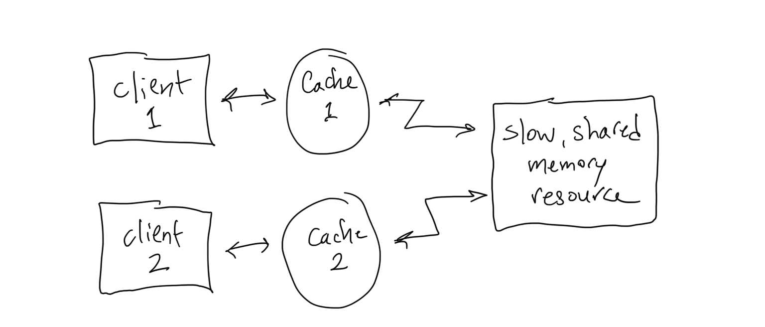
Reads to a coherent cache always read data that is at least as new as the underlying storage. That is, a coherent cache provides the same semantics as direct access to the underlying storage.
An incoherent cache does not always provide its read users with the most up-to-date view of underlying storage. In particular, an incoherent cache can return stale data, data that does not represent the latest values written to a set of addresses.
The coherence.cc program demonstrates that the stdio cache is incoherent:
the stdio library does not update the data in its cache associated with a
particular FILE pointer even when the same program uses the stdio library to
write to the same file on disk, but using a different FILE pointer.
The buffer cache is coherent, however. Every access to the disk is made through the operating system kernel, through system calls, and an important part of the kernel’s job is to ensure that the buffer cache is kept coherent—that write system calls made by one application are visible to system calls made by other applications as soon as those writes are made.
You can force the stdio cache to become coherent by adding a fflush(f) call
before every read. This call flushes any cached read data, in addition to
flushing out any buffered writes. But then stdio isn’t much of a cache!
The processor cache is also coherent (up to the limitations of the machine’s memory model, an advanced topic).
Note that a cache still counts as coherent according to this definition if some cached data, somewhere in the system, is newer than the underlying storage—that is, if writes are being buffered. Coherence is a read property.
The stdio application interface does give applications some control over its
coherence. Applications can request that stdio not cache a given file with
setvbuf(3).
Clean and dirty slots
Data in a read cache is sometimes in sync with underlying storage, and sometimes—if the cache is incoherent—that data is older than underlying storage. By older, we mean that the cache holds values that were once held (at an earlier time) in memory, but are not currently held in memory.
Conversely, sometimes a processor has written data into a cache and this value has not yet made its way to the underlying storage. We say that this cache contains data that is newer than underlying storage. This newer data was written at a time later than the write that is in the underlying slow storage. This can happen if a write cache is coalescing writes or batching, and the cache has not yet written these batched writes to the underlying slower storage.
A cache slot that contains data newer than underlying storage is called dirty. A slot containing data that is not newer than underlying storage is called clean. A clean slot in an incoherent cache may be older than the underlying storage. Also, by definition, an empty slot is considered clean because it never needs to be flushed to the underlying storage.
For an example of both incoherent caches and dirty slots, consider the
following steps involving a single file, f.txt, that’s opened twice
by stdio, once for reading and once for writing. (Either the same
program called fopen twice on the same file, or two different
programs called fopen on the same file.) The first column shows the
buffer cache’s view of the file, which is coherent with the underlying
disk. The other two show the stdio caches’ views of the file. The file
initially contains all “A”s.
| Buffer cache | Stdio cache f1 | Stdio cache f2 | |
|---|---|---|---|
1. Initial state of f.txt |
“AAAAAAAAAA” | ||
2. f1 = fopen("f.txt", "r") |
“AAAAAAAAAA” | (empty) | |
3. fgetc(f1) |
“AAAAAAAAAA” | “AAAAAAAAAA” | |
4. f2 = fopen("f.txt", "w") |
“AAAAAAAAAA” | “AAAAAAAAAA” | (empty) |
5. fprintf(f2, "BB…") |
“AAAAAAAAAA” | “AAAAAAAAAA” | “BBBBBBBBBB” |
6. fflush(f2) |
“BBBBBBBBBB” | “AAAAAAAAAA” | (empty) |
At step 5, after fprintf but before fflush, f2’s stdio cache is dirty: it
contains newer data than underlying storage. At step 6, after fflush, f1’s
stdio cache demonstrates incoherence: it contains older data than underlying
storage. At steps 2–4, though, f1’s stdio cache is clean and coherent.
A write-through cache is designed to never contain dirty slots. As such, write-through caches do not perform write coalescing or batching for writes: every write to the cache goes immediately “through” to underlying storage. Such caches are still useful for reads.
In contrast, a write-back cache coalesces and batches writes. This means that this type of cache can contain dirty slots, which are lazily written to the underlying slower storage. As you saw in the pset, dirty slots are flushed when we need to use the slot for new data, or when the processor forces all dirty slots to be written to the underlying slower storage.
The stdio cache is a write-back cache, and fclose forces a flush of
all dirty slots corresponding to the closed FILE pointer. The
buffer cache acts like a write-through cache for any file opened with
the O_SYNC flag.